


The Poynting vectors, spin and orbital angular momentums of uniformly polarized cosh-Pearcey-Gauss beams in the far zone
doi: 10.37188/CO.EN.2022-0022
-
摘要:
本文提出了均匀偏振cosh-Pearcey-Gauss 光束,其主要由双曲余弦函数(
n ,Ω )和偏振相关角度(α ,δ )所调制。基于矢量角谱法和稳相法,研究了该光束的远场坡印廷矢量、自旋角动量和轨道角动量。研究结果表明:较大的双曲余弦函数值能将远场坡印廷矢量、自旋角动量和轨道角动量分割成多瓣抛物线结构。虽然左旋和右旋椭圆偏振不能影响整个光束结构,但却可通过调节TE和TM项的左半边和右半边的分布权重,进而分辨出光束的远场坡印廷矢量和角动量分布。本文结果对信息存储与偏振成像技术领域有着潜在的应用价值。-
关键词:
- cosh-Pearcey-Gauss光束 /
- 自旋角动量 /
- 轨道角动量 /
- 坡印廷矢量
Abstract:We propose cosh-Pearcey-Gauss beams with uniform polarization, which are mainly modulated by a hyperbolic cosine function (
n ,Ω ) and the angles related to uniform polarization (α ,δ ). Based on angular spectrum representation and the stationary phase method, the Poynting vector, Spin Angular Momentums (SAM) and Orbital Angular Momentums (OAMs) in the far zone are studied. The results show that a largern orΩ in the hyperbolic cosine function can partition the longitudinal Poynting vectors, SAMs and OAMs into more multi-lobed parabolic structures. Different polarizations described by (α ,δ ) can distinguish their Poynting vectors and angular momentums between the TE and TM terms, though this does not affect the patterns of the whole beam. Furthermore, the weight of the left and right sides of longitudinal Poynting vectors, SAMs and OAMs in TE and TM terms can be modulated by left-handed or right-handed elliptical polarization, respectively. The results in this paper may be useful for information storage and polarization imaging. -
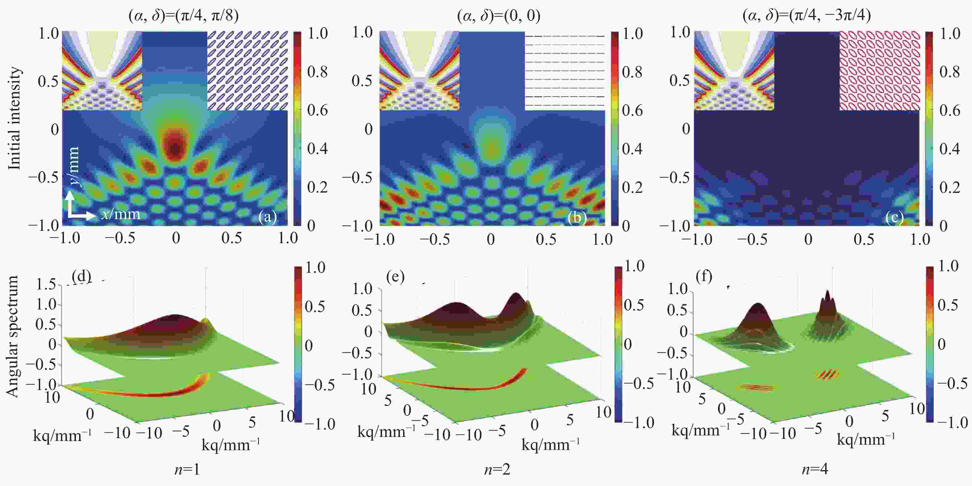
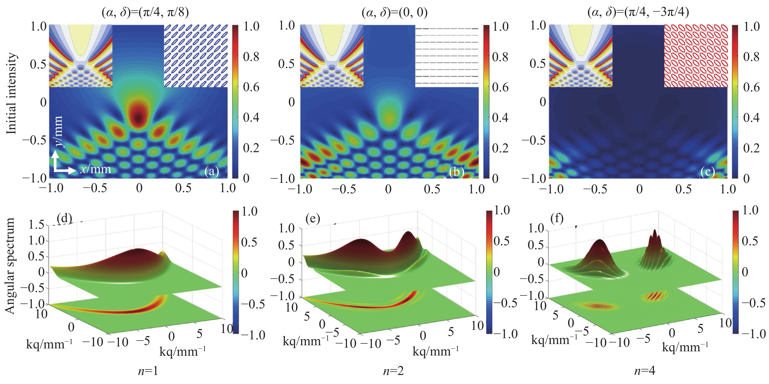
Figure 1. The initial intensities and angular spectra of the cPeG beams with different initial polarization states for n=1, 2 and 4. (a), (d): α=π/4, δ=π/8; (b), (e): α=0, δ=0; (c), (f): α=π/4, δ=−3π/4. The phase distribution and polarization states are described in the top form left to right in Figs.1 (a)−(c). Blue: left-handed elliptical polarization; Red: right-handed elliptical polarization; Black: linear polarization. The parameters are x0=y0=100 μm and Ω=1.4

Figure 2. The theoretical design scheme of the cPeG beams with uniform polarization. BS: Beam Splitter; SLM: Spatial Light Modulator

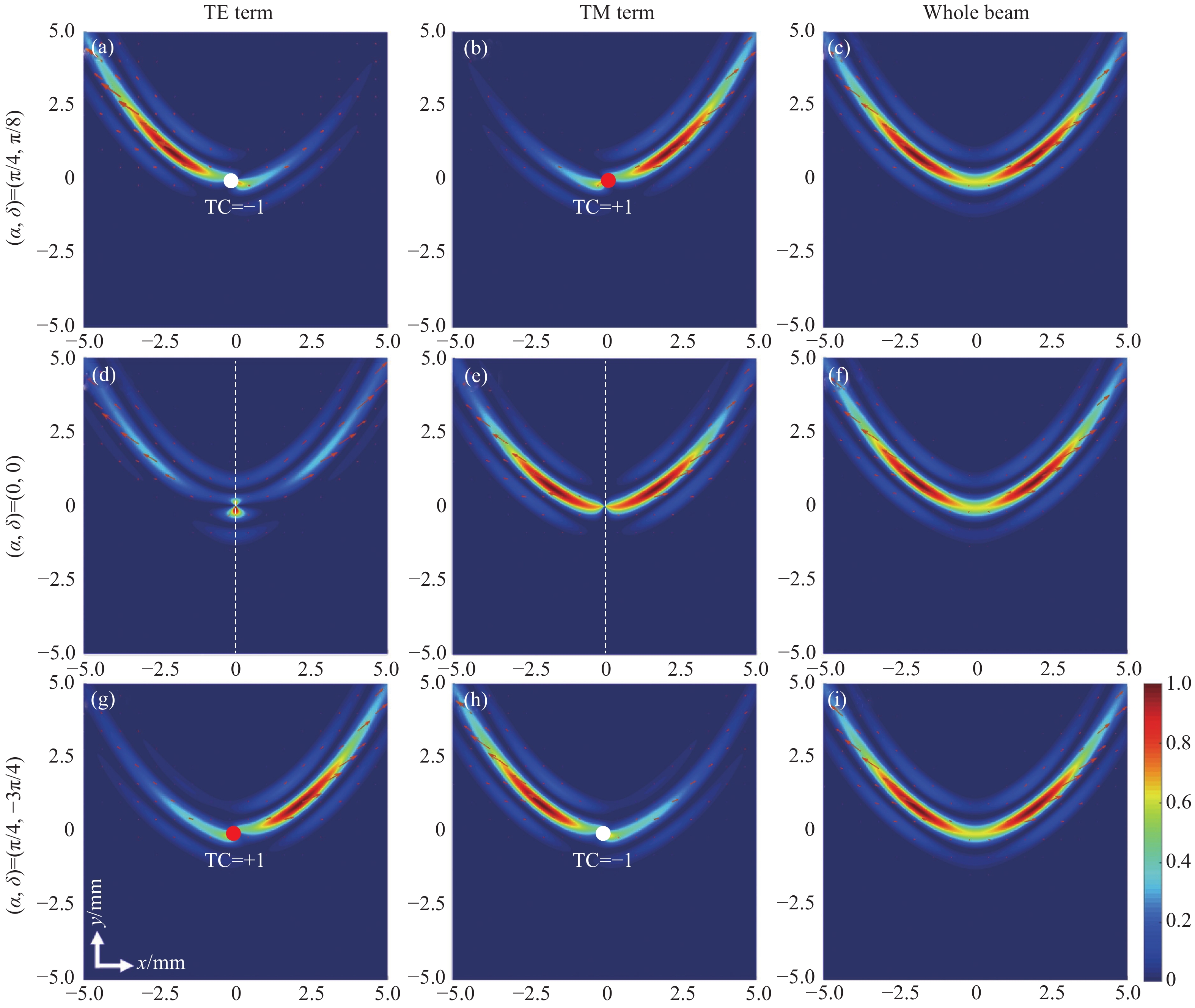
Figure 3. Normalized longitudinal Poynting vector (backgrounds) and transversal Poynting vector (arrows) of cPeG beams for different uniform polarizations (α, δ) at z=50z0. (a), (d), (g): TE term; (b), (e), (h): TM term; (c), (f), (i): whole beam. The parameters are n=2 and Ω=1.4. The red point symbolizes topological charge l=+1, and the white point denotes l=−1
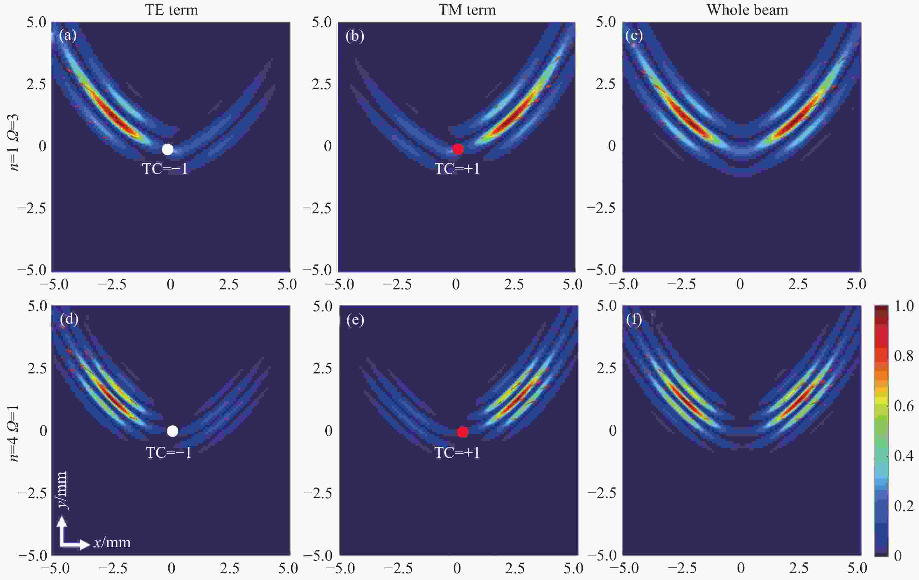
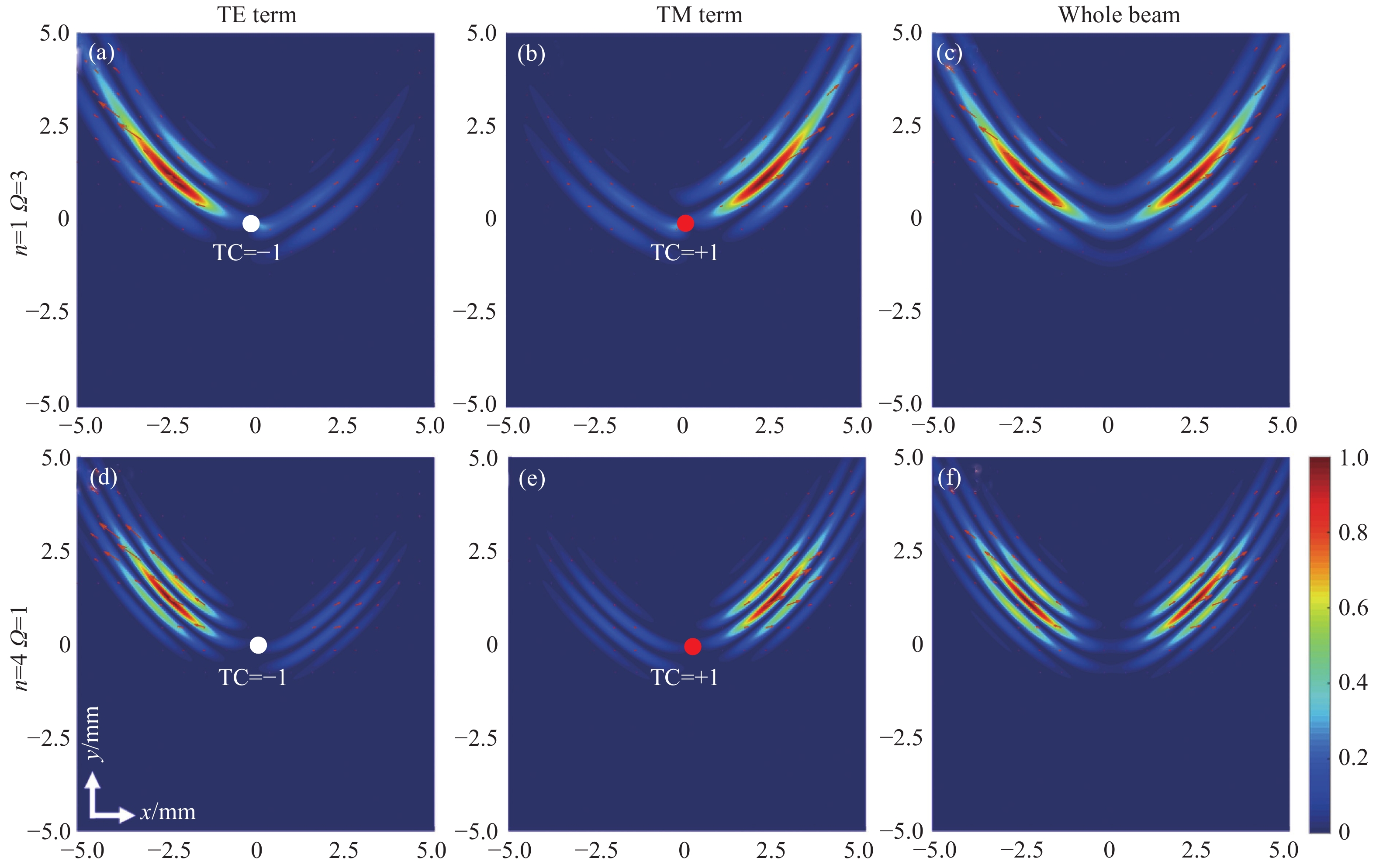
Figure 4. Normalized longitudinal Poynting vector (backgrounds) and transverse Poynting vector (arrows) of cPeG beams for different n and Ω at z=50z0, where the uniform polarization is (α, δ)=(π/4,π/8)

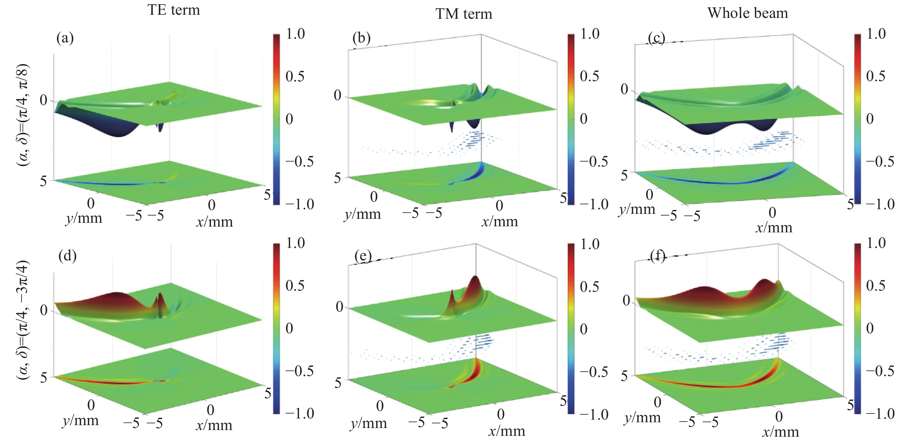
Figure 5. Normalized longitudinal SAM (3D and 2D) and transverse SAM (arrows) of cPeG beams at z=50z0. (a)−(c): α=π/4, δ=π/8; (d)−(f): α=π/4, δ=−3π/4. The other parameters are the same as those in Fig. 3

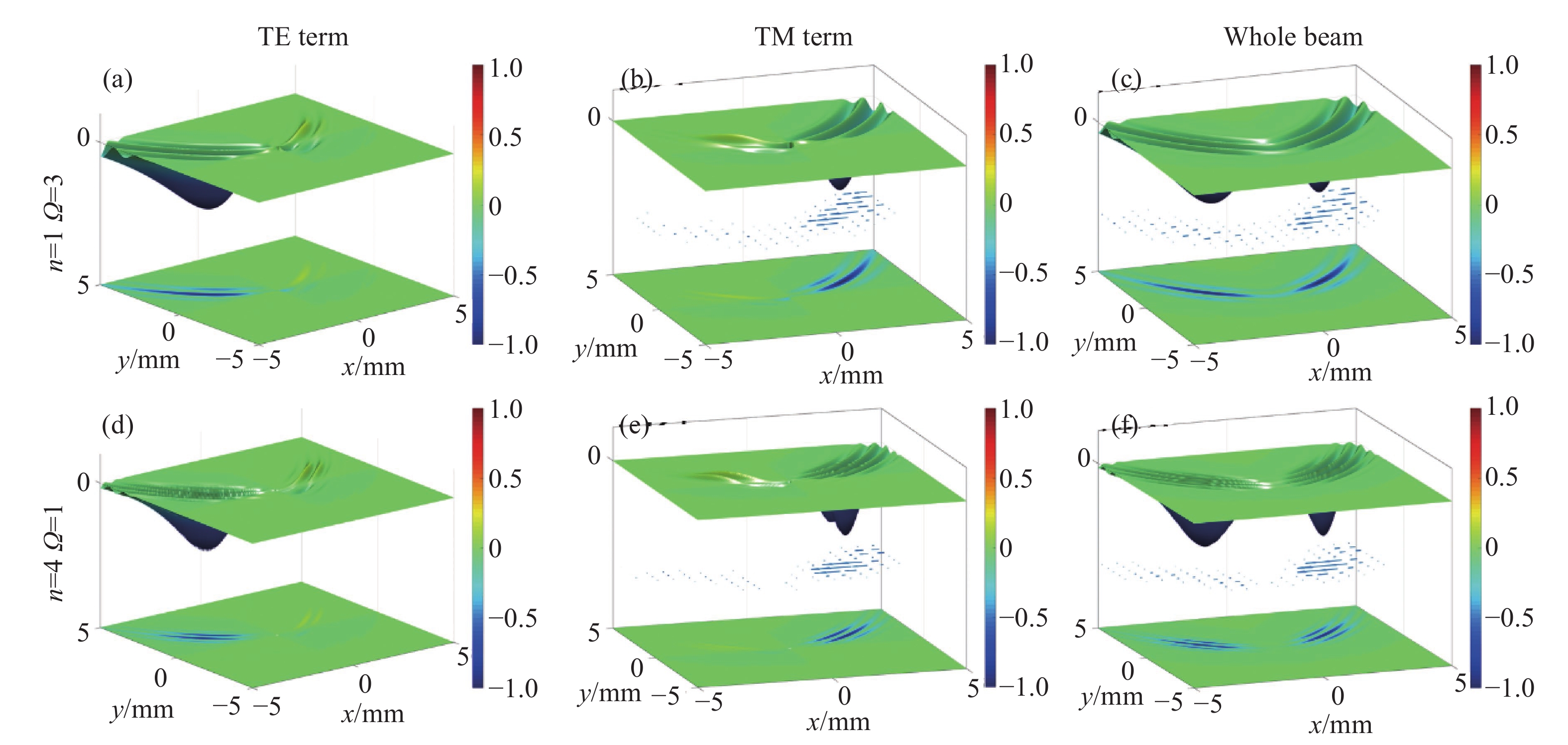
Figure 6. Normalized longitudinal (3D and 2D) SAM and transverse SAM (arrows) of cPeG beams (n=1, 4) at z=50z0. (a)−(c): n=1, Ω=3; (d)−(f): n=4, Ω=1. The other parameters are the same as those in Figs. 5 (α=π/4, δ=π/8)

Figure 7. Normalized longitudinal OAM (3D and 2D) and transverse OAM (arrows) of cPeG beams (Ω=1.4) at z=50z0. (a)−(c): α=π/4, δ=π/8; (d)-(f): α= 0, δ= 0; (g)−(i): α=π/4, δ=−3π/4; The other parameters are the same as those in Fig. 3. (n=2)
-
[1] PEARCEY T. XXXI. The structure of an electromagnetic field in the neighbourhood of a cusp of a caustic[J]. The London,Edinburgh,and Dublin Philosophical Magazine and Journal of Science, 1946, 37(268): 311-317. doi: 10.1080/14786444608561335 [2] RING J D, LINDBERG J, MOURKA A, et al. Auto-focusing and self-healing of Pearcey beams[J]. Optics Express, 2012, 20(17): 18955-18966. doi: 10.1364/OE.20.018955 [3] KOVALEV A A, KOTLYAR V V, ZASKANOV S G, et al. Half Pearcey laser beams[J]. Journal of Optics, 2015, 17(3): 035604. doi: 10.1088/2040-8978/17/3/035604 [4] REN ZH J, LI X D, JIN H ZH, et al. Construction of Bi-Pearcey beams and their mathematical mechanism[J]. Acta Physica Sinica, 2016, 65(21): 214208. doi: 10.7498/aps.65.214208 [5] LIU Y J, XU CH J, LIN Z J, et al. Auto-focusing and self-healing of symmetric odd-Pearcey Gauss beams[J]. Optics Letters, 2020, 45(11): 2957-2960. doi: 10.1364/OL.394443 [6] GAO R, REN SH M, GUO T, et al. Propagation dynamics of chirped Pearcey-Gaussian beam in fractional Schrödinger equation under Gaussian potential[J]. Optik, 2022, 254: 168661. doi: 10.1016/j.ijleo.2022.168661 [7] CHEN K H, QIU H X, WU Y, et al. Generation and control of dynamically tunable circular Pearcey beams with annular spiral-zone phase[J]. Science China Physics,Mechanics &Astronomy, 2021, 64(10): 104211. [8] ZHOU X Y, PANG Z H, ZHAO D M. Generalized ring pearcey beams with tunable autofocusing properties[J]. Annalen der Physik, 2021, 533(7): 2100110. doi: 10.1002/andp.202100110 [9] NOSSIR N, DALIL-ESSAKALI L, BELAFHAL A. Diffraction of generalized Humbert–Gaussian beams by a helical axicon[J]. Optical and Quantum Electronics, 2021, 53(2): 94. doi: 10.1007/s11082-020-02662-5 [10] ZHAO X L, JIA X T. Vectorial structure of arbitrary vector vortex beams diffracted by a circular aperture in the far field[J]. Laser Physics, 2018, 28(1): 015004. doi: 10.1088/1555-6611/aa9813 [11] CHENG K, LU G, ZHONG X Q. Energy flux density and angular momentum density of radial Pearcey-Gauss vortex array beams in the far field[J]. Optik, 2017, 149: 189-197. doi: 10.1016/j.ijleo.2017.09.032 [12] SHU L Y, CHENG K, LIAO S, et al. Spin angular momentum flux density of non-uniformly polarized vortex beams with tunable polarization angles in uniaxial crystals[J]. Optik, 2021, 243: 167464. doi: 10.1016/j.ijleo.2021.167464 [13] YANG Q SH, XIE Z J, ZHANG M R, et al. Ultra-secure optical encryption based on tightly focused perfect optical vortex beams[J]. Nanophotonics, 2022, 11(5): 1063-1070. doi: 10.1515/nanoph-2021-0786 [14] ZHU L W, CAO Y Y, CHEN Q Q, et al. Near-perfect fidelity polarization-encoded multilayer optical data storage based on aligned gold nanorods[J]. Opto-Electronic Advances, 2021, 4(11): 210002. doi: 10.29026/oea.2021.210002 [15] OUYANG X, XU Y, XIAN M C, et al. Synthetic helical dichroism for six-dimensional optical orbital angular momentum multiplexing[J]. Nature Photonics, 2021, 15(12): 901-907. doi: 10.1038/s41566-021-00880-1 [16] ALLEN L, BARNETT S M, PADGETT M J. Optical Angular Momentum[M]. Boca Raton: CRC Press, 2003. [17] BAI Y H, LV H R, FU X, et al. Vortex beam: generation and detection of orbital angular momentum [Invited][J]. Chinese Optics Letters, 2022, 20(1): 012601. doi: 10.3788/COL202220.012601 [18] WU G H, LOU Q H, ZHOU J. Analytical vectorial structure of hollow Gaussian beams in the far field[J]. Optics Express, 2008, 16(9): 6417-6424. doi: 10.1364/OE.16.006417 [19] CHENG K, LIANG M T, SHU L Y, et al. Polarization states and Stokes vortices of dual Butterfly-Gauss vortex beams with uniform polarization in uniaxial crystals[J]. Optics Communications, 2022, 504: 127471. doi: 10.1016/j.optcom.2021.127471 [20] ZHOU G Q, NI Y ZH, ZHANG ZH W. Analytical vectorial structure of non-paraxial nonsymmetrical vector Gaussian beam in the far field[J]. Optics Communications, 2007, 272(1): 32-39. doi: 10.1016/j.optcom.2006.11.044 [21] ZHOU G Q. Vectorial structure of an apertured Gaussian beam in the far field: an accurate method[J]. Journal of the Optical Society of America A, 2010, 27(8): 1750-1755. doi: 10.1364/JOSAA.27.001750 [22] MANDEL L, WOLF E. Optical Coherence and Quantum Optics[M]. Cambridge: Cambridge University Press, 1995. [23] GU B, WEN B, RUI G H, et al. Varying polarization and spin angular momentum flux of radially polarized beams by anisotropic Kerr media[J]. Optics Letters, 2016, 41(7): 1566-1569. doi: 10.1364/OL.41.001566 [24] ANDREWS D L, BABIKER M. The Angular Momentum of Light[M]. Cambridge: Cambridge University Press, 2012. [25] CHEN R P, CHEW K H, DAI C Q, et al. Optical spin-to-orbital angular momentum conversion in the near field of a highly nonparaxial optical field with hybrid states of polarization[J]. Physical Review A, 2017, 96(5): 053862. doi: 10.1103/PhysRevA.96.053862 -
-

 下载:
下载:


计量
- 文章访问数: 1106
- HTML全文浏览量: 841
- PDF下载量: 230
- 被引次数: 0
