


Influence of sampling on three-dimensional surface shape measurement
doi: 10.37188/CO.EN-2024-0003
-
摘要:
本文研究了抽样对三维形貌测量的影响。首先,利用傅立叶变换推出频谱表达式。在此基础上,分析了CCD像元的产生过程并给出了其表达式。然后,经抽样得到离散的变形条纹表达式,并推导出了其傅立叶频谱表达式,从而得到频域内无限重复的“频谱岛”。 最后,利用低通滤波器滤除高级频谱成份后仅保留其中一个基频成份,由逆傅立叶变换恢复信号强度。提出减小抽样间隔,即减小每根条纹抽样点数的方法,来增大抽样频率与光栅基频的比值
m ,使之在满足m >4的条件下能更准确地恢复物体的三维形貌。通过仿真和实验对基本原理进行验证。在仿真分析中,抽样间隔分别取8 pixels、4 pixels、2 pixels、1 pixel,后3种情况所得到的最大绝对误差值分别为第一种情况下的88.80%、38.38%和31.50%,平均绝对误差值分别为第一种情况下的71.84%、43.27%和32.26%。可见,抽样间隔越小,恢复效果越好。在实验中,取与仿真分析相同的4次抽样间隔,得到了与仿真分析相同的结论。结果表明:减小抽样间隔可提高三维形貌的测量精度,取得了更好的恢复效果。Abstract:In order to accurately measure an object’s three-dimensional surface shape, the influence of sampling on it was studied. First, on the basis of deriving spectra expressions through the Fourier transform, the generation of CCD pixels was analyzed, and its expression was given. Then, based on the discrete expression of deformation fringes obtained after sampling, its Fourier spectrum expression was derived, resulting in an infinitely repeated "spectra island" in the frequency domain. Finally, on the basis of using a low-pass filter to remove high-order harmonic components and retaining only one fundamental frequency component, the inverse Fourier transform was used to reconstruct the signal strength. A method of reducing the sampling interval, i.e., reducing the number of sampling points per fringe, was proposed to increase the ratio
$ m $ between the sampling frequency and the fundamental frequency of the grating. This was done to reconstruct the object’s surface shape more accurately under the condition of$m > 4$ . The basic principle was verified through simulation and experiment. In the simulation, the sampling intervals were 8 pixels, 4 pixels, 2 pixels, and 1 pixel, the maximum absolute error values obtained in the last three situations were 88.80%, 38.38%, and 31.50% in the first situation, respectively, and the corresponding average absolute error values are 71.84%, 43.27%, and 32.26%. It is demonstrated that the smaller the sampling interval, the better the recovery effect. Taking the same four sampling intervals in the experiment as in the simulation can also lead to the same conclusions. The simulated and experimental results show that reducing the sampling interval can improve the accuracy of object surface shape measurement and achieve better reconstruction results. -
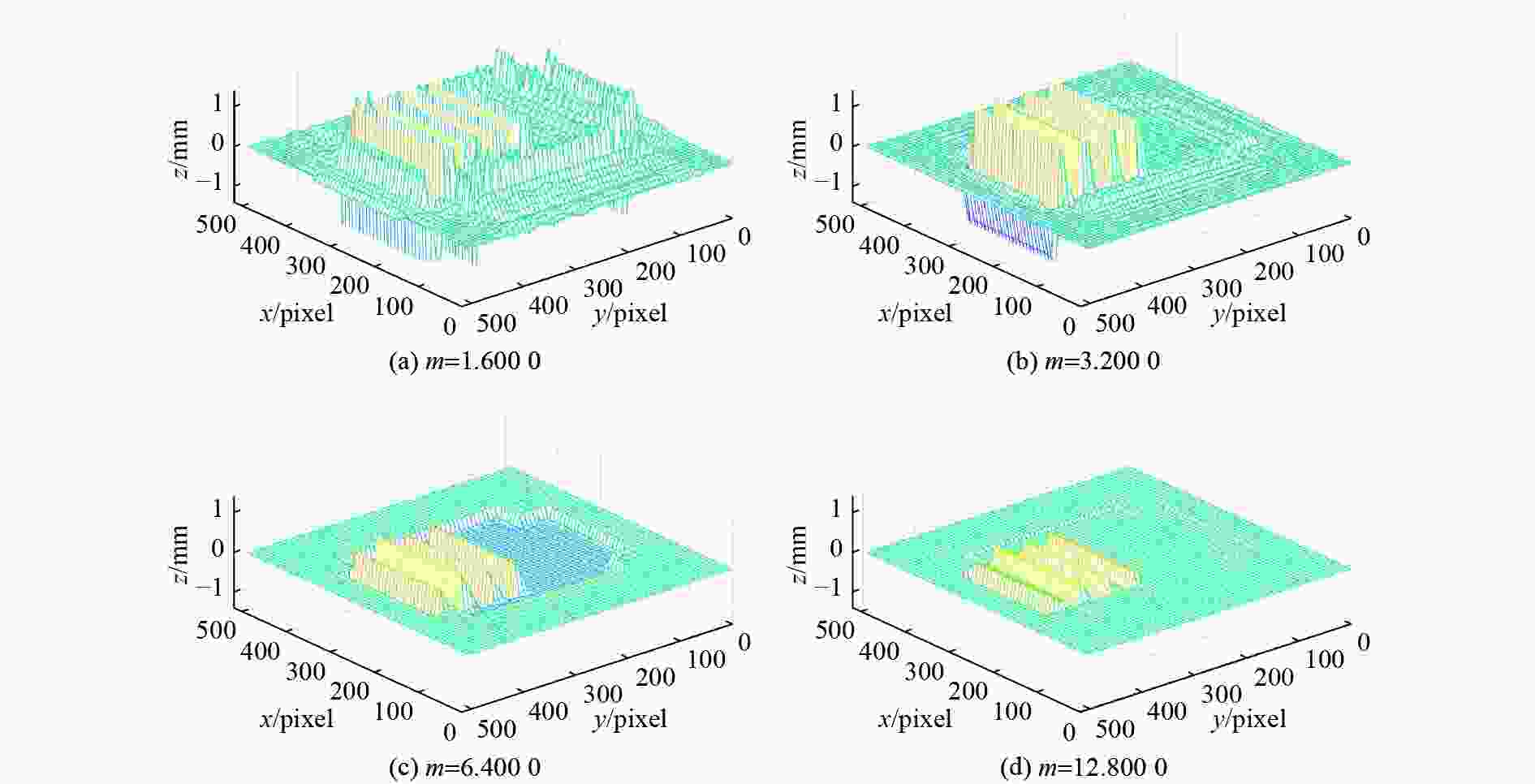
Figure 4. The errors in the surface shape between the reconstructed and simulated objects
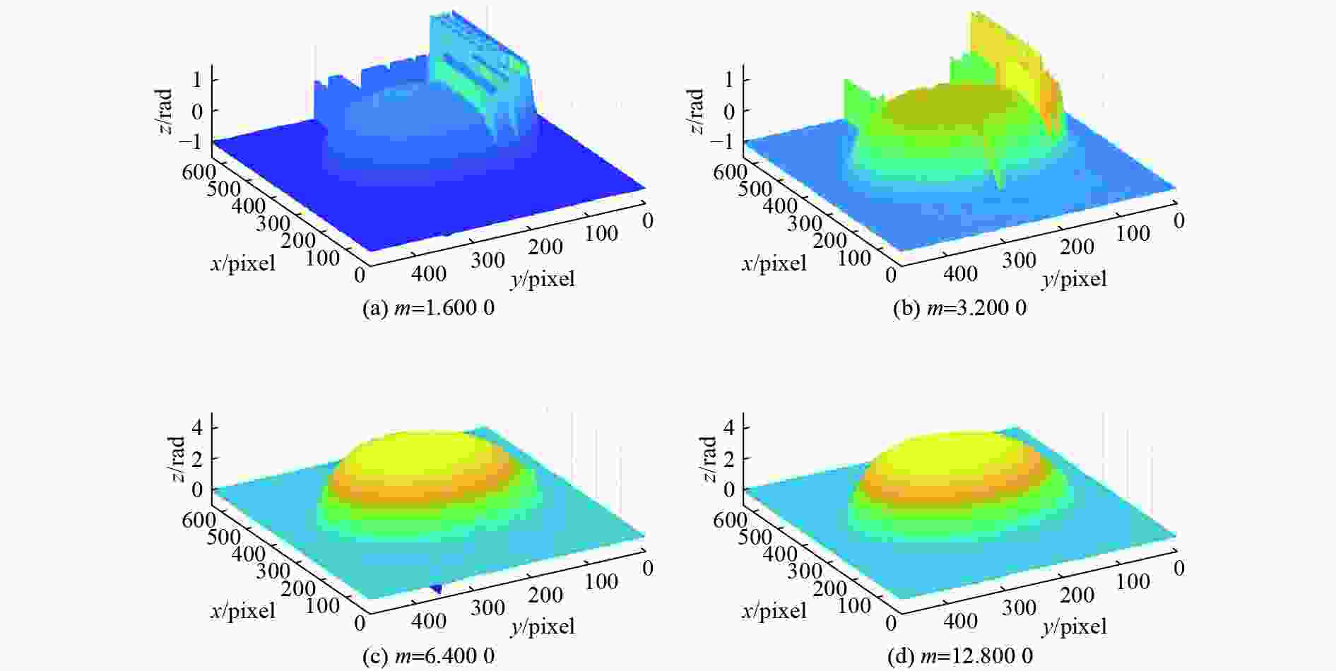
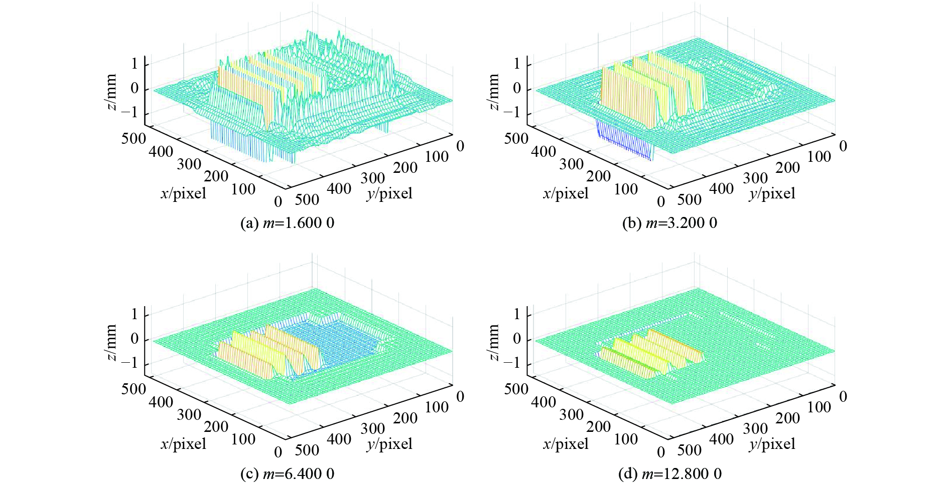
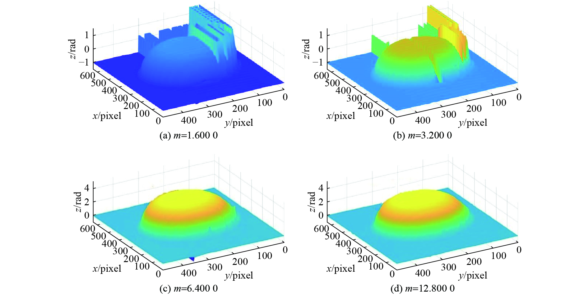
Figure 6. Results of object surface shape reconstructed under different sampling conditions
Table 1. Error between reconstructed object and simulated object
Sampling interval 8 pixels 4 pixels 2 pixels 1 pixels MAEV 1.3246 1.1762 0.5084 0.4173 AAEV 0.4758 0.3418 0.2059 0.1535  下载: 导出CSV
-
[1] MA X X, NI H, LU M SH, et al. A measurement method for three-dimensional inner and outer surface profiles and spatial shell uniformity of laser fusion capsule[J]. Optics & Laser Technology, 2021, 134: 106601. [2] FAN H, QI L, CHEN CH H, et al. Underwater optical 3-D reconstruction of photometric stereo considering light refraction and attenuation[J]. IEEE Journal of Oceanic Engineering, 2022, 47(1): 46-58. doi: 10.1109/JOE.2021.3085968 [3] YANG J B, ZHAO J, SUN Q. Projector calibration based on cross ratio invariance[J]. Chinese Optics, 2021, 14(2): 320-328. (in Chinese). doi: 10.37188/CO.2020-0111 [4] ZHOU P, WANG H Y, LAI J L, et al. 3D shape measurement for shiny surface using pixel-wise composed fringe pattern based on multi-intensity matrix projection of neighborhood pixels[J]. Optical Engineering, 2021, 60(10): 104101. [5] YANG SH CH, HUANG H L, WU G X, et al. High-speed three-dimensional shape measurement with inner shifting-phase fringe projection profilometry[J]. Chinese Optics Letters, 2022, 20(11): 112601. doi: 10.3788/COL202220.112601 [6] LU L L, WU ZH J, ZHANG Q C, et al. High-efficiency dynamic three-dimensional shape measurement based on misaligned gray-code light[J]. Optics and Lasers in Engineering, 2022, 150: 106873. doi: 10.1016/j.optlaseng.2021.106873 [7] FENG W, XU SH N, WANG H H, et al. Three-dimensional measurement method of highly reflective surface based on per-pixel modulation[J]. Chinese Optics, 2022, 15(3): 488-497. (in Chinese). doi: 10.37188/CO.2021-0220 [8] QIAO N SH, ZHANG F. Method for reducing phase errors due to CCD nonlinearity[J]. Optik, 2016, 127(13): 5207-5210. doi: 10.1016/j.ijleo.2016.03.012 [9] LIU H Q, MA H M, TANG Q X, et al. Investigation of noise amplification questions in satellite jitter detected from CCDs' parallax observation imagery: a case for 3 CCDs[J]. Optics Communications, 2022, 503: 127422. doi: 10.1016/j.optcom.2021.127422 [10] XUE X, ZHANG CH M, ZHAO J K, et al. The influence of CCD undersampling on the encircled energy of SVOM-VT[J]. Proceedings of the SPIE, 2019, 11341: 1134104. [11] DU Y ZH, FENG G Y, ZHANG K, et al. Effect of CCD nonlinearity on wavefront detection by shearing interferometry[J]. High Power Laser and Particle Beams, 2010, 22(8): 1775-1779. doi: 10.3788/HPLPB20102208.1775 [12] CHENG SH B, ZHANG H G, WANG ZH B, et al. Nonlinearity property testing of the scientific grade optical CCD[J]. Acta Optica Sinica, 2012, 32(4): 0404001. (in Chinese). doi: 10.3788/AOS201232.0404001 [13] QIAO N SH, SUN P. Influence of CCD nonlinearity effect on the three-dimensional shape measurement of dual frequency grating[J]. Chinese Optics, 2021, 14(3): 661-669. (in Chinese). doi: 10.37188/CO.2020-0143 [14] LI J, SU X Y, GUO L R. Improved Fourier transform profilometry for the automatic measurement of three-dimensional object shapes[J]. Optical Engineering, 1990, 29(12): 1439-1444. [15] QIAO N SH. Effect of CCD nonlinearity on spectrum distribution[J]. Optik, 2016, 127(20): 8607-8612. doi: 10.1016/j.ijleo.2016.06.070 [16] WANG Y, LIN B. A fast and precise three-dimensional measurement system based on multiple parallel line lasers[J]. Chinese Physics B, 2021, 30(2): 024201. doi: 10.1088/1674-1056/abc14d [17] SUN J H, ZHANG Q Y. A 3D shape measurement method for high-reflective surface based on accurate adaptive fringe projection[J]. Optics and Lasers in Engineering, 2022, 153: 106994. doi: 10.1016/j.optlaseng.2022.106994 [18] CAO ZH R. Dynamic 3D measurement error compensation technology based on phase-shifting and fringe projection[J]. Chinese Optics, 2023, 16(1): 184-192. (in Chinese). doi: 10.37188/CO.EN.2022-0004 [19] QIAO N SH, SHANG X. Phase measurement with dual-frequency grating in a nonlinear system[J]. Chinese Optics, 2023, 16(3): 726-732. (in Chinese). doi: 10.37188/CO.EN.2022-0013 -


 下载:
下载:

计量
- 文章访问数: 194
- HTML全文浏览量: 84
- PDF下载量: 127
- 被引次数: 0
