


Range limited adaptive brightness preserving multi-threshold histogram equalization algorithm
doi: 10.3788/CO.20171006.0726
-
摘要: 针对目前直方图均衡算法难以实现,且易造成亮度饱和等问题,本文提出了一种范围限制的自适应亮度保持多阈值直方图均衡算法。首先,对输入图像进行适当平滑,从而获得它的直方图峰值点个数(N+1)。然后,对Otsu算法进行N阈值扩展,并通过这种方法获得图像的N个分割阈值,从而按照此阈值对图像进行分割。为了能够最大程度地保持输入图像的亮度,利用输入图像和输出图像的均值亮度最小误差(AMBE)准则,重新计算了图像的均衡范围。最后,利用新的均衡范围分别对每一个子图像进行均衡。实验表明,使用本算法处理Lena图的绝对均值亮度误差为0.416 4,明显优于使用RLBHE算法的0.629 5。本算法能够获得更清晰的图像细节,同时图像的整体亮度保持的也较好。Abstract: In recent years, many histogram equalization algorithms have been proposed for the consumer electronics field. However, many of these algorithms are hard to realize. Even, for example, some algorithms may cause an effect on brightness saturation. Therefore, a range limited adaptive brightness preserving multi-threshold histogram equalization(RLAMHE) algorithm is presented in this paper. First, the input image is smoothed appropriately to obtain the number of its histogram peak points (N+1). Then the Otsu algorithm is extended by the N-threshold, and N segmentation thresholds of the image are obtained in this way, so that the image is segmented according to this threshold. In order to maximize the brightness of the input image, a range of the equalized image is recalculated according to the minimum Absolute Mean Brightness Error(AMBE) criterion of the input and the output image. Finally, all sub-images are equalized separately using the new equalization range. Test results show that the proposed algorithm is more efficient than other algorithms and can obtain sharper image details. Meanwhile, the overall brightness of the image is also ideal. Using this algorithm to process Lena graphs, the absolute mean luminance error is 0.416 4, which is obviously better than that obtained using RLBHE algorithm(0.629 5).
-
Key words:
- contrast enhancement /
- histogram equalization /
- brightness preserving /
- range limited /
- N-threshold
-

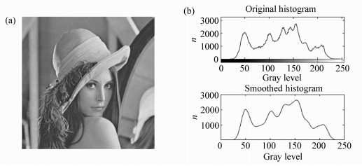
Figure 1. (a) Original image of Lena. (b)Comparison of the original histogram and the smoothed one of Fig. 1(a)

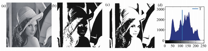
Figure 2. (a) Original image of Lena. (b), (c)Separation results using the single threshold Otsu′s method. (d)Location of threshold using the single threshold Otsu′s method

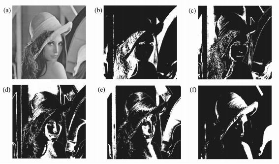
Figure 4. (a) Original image of Lena.(b)~(f)Separation results using the N-threshold Otsu′s method

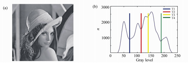
Figure 3. (a) Original image of Lena. (b)Location of thresholds using the N-threshold Otsu′s method

Figure 5. (a) Original image of Lena.(b)Result of GHE.(c) Result of RLBHE.(d) Result of RLAMHE

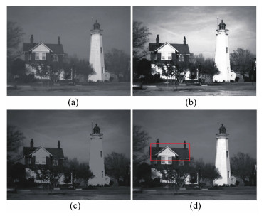
Figure 6. (a) Original image of House.(b)Result of GHE.(c) Result of RLBHE.(d) Result of RLAMHE

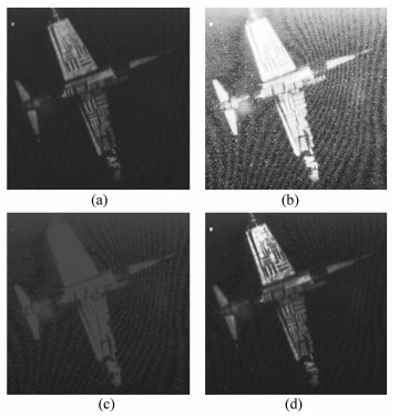
Figure 7. (a) Original image of Airplane U2.(b)Result of GHE.(c) Result of RLBHE.(d) Result of RLAMHE
Table 1. The resulting AMBE for GHE, RLBHE and RLAMHE
GHE RLBHE RLAMHE Lena 3.250 1 0.629 5 0.414 6 House 70.008 8 7.116 6 2.954 2 AirplaneU2 94.997 9 5.963 2 1.339 8  下载: 导出CSV
-
[1] CHEN H O, NICHOLAS S P K, HAIDI I. Bi-histogram equalization with a plateau limit for digital image enhancement[J]. IEEE Trans. Consum. Electron, 2009, 55:2072-2080. doi: 10.1109/TCE.2009.5373771 [2] MENOTTI D, NAJMAN L, FACON J, et al.. Multi-hirtogram equalization methods for contrast enhancement and brightness preserving[J]. IEEE Trans. Consum. Electron, 2007, 53:1186-1194. doi: 10.1109/TCE.2007.4341603 [3] KIM Y T. Contrast enhancement using brightness preserving bi-histogram equalization[J]. IEEE Trans. Consum. Electron, 1997, 43:1-8. doi: 10.1109/30.580378 [4] WAN Y, CHEN Q, ZHANG B M. Image enhancement based on equal area dualistic sub-image histogram equalization method[J]. IEEE Trans. Consum. Electron, 1999, 45:68-75. doi: 10.1109/30.754419 [5] CHEN S D, RAMLI A R. Minimum mean brightness error bi-histogram equalization in contrast enhancement[J]. IEEE Trans. Consum. Electron, 2003, 49:1310-1319. doi: 10.1109/TCE.2003.1261234 [6] SIM K S, TSO C P, TAN Y Y. Recursive sub-image histogram equalization applied to gray scale images[J]. Pattern Recognit. Lett., 2007, 28:1209-1221. http://www.sciencedirect.com/science/article/pii/S0167865507000578 [7] ZUO CH, CHEN Q, SUI X B. Range limited bi-histogram equalization for image contrast enhancement[J]. Optik, 2013, 124:425-431. doi: 10.1016/j.ijleo.2011.12.057 [8] WANG CH, YE ZH F. Brightness preserving histogram equalization with maximum entropy:a variational perspective[J]. IEEE Trans. Consum. Electron, 2005, 51:1326-1334. http://ieeexplore.ieee.org/xpls/icp.jsp?arnumber=1561863 [9] XIU CH B, WEI SH A N. Camshift tracking with saliency histogram[J]. Optics and Precision Engineering, 2015, 23(6):1749-1757. http://www.opticsjournal.net/Abstract.htm?id=OJ1508250005958EaGdJ [10] LI Y, ZHANG Y F, NIAN L, et al.. [J]. Chinese J. Liquid Crystals and Displays, 2016, 31(1):104-111.(in Chinese) http://www.opticsjournal.net/abstract.htm?id=OJ160322000625x5A7D0 [11] ZHOU Y, LI Q W, HUO G Y. Adaptive image enhancement based on NSCT coefficient histogram matching[J]. Optics and Precision Engineering, 2014, 22(8):2215-2222.(in Chinese) http://en.cnki.com.cn/Article_en/CJFDTotal-GXJM201408032.htm [12] XIAO CH M, SHI Z L, LIU Y P. Metrics of image background clutter by introducing gradient features[J]. Optics and Precision Engineering, 2015, 23(12):3472-3479.(in Chinese) http://www.opticsjournal.net/abstract.htm?id=OJ160122000089jPlSoV [13] CAO J F, SHI J CH, LUO H B, et al.. Image enhancement using clustering and histogram equalization[J]. Infrared and Laser Engineering, 2012, 41(12):3436-3441.(in Chinese) http://en.cnki.com.cn/Article_en/CJFDTOTAL-HWYJ201212052.htm [14] YUN H J, WU ZH Y, WANG G J, et al.. Enhancement of infrared image combined with histogram equalization and fuzzy set theory[J]. J. Computer-Aided Design & Computer Graphics, 2015, 27(8):1498-1505.(in Chinese) [15] CHEN Y, ZHU M. Multiple sub-histogram equalization low light level image enhancement and realization on FPGA[J]. Chinese J. Optics, 2014, 7(2):225-233.(in Chinese) http://en.cnki.com.cn/Article_en/CJFDTotal-ZGGA201402006.htm [16] CAI SH D, YANG F. Image enhancement based on histogram modification[J]. Optoeletronic Technology, 2012, 32(3):155-159.(in Chinese) http://en.cnki.com.cn/Article_en/CJFDTOTAL-GDJS201203004.htm -

 下载:
下载:


计量
- 文章访问数: 2488
- HTML全文浏览量: 790
- PDF下载量: 506
- 被引次数: 0
